
Understanding Normal Distribution
The normal distribution is the well-known bell-shaped curve depicted below. The bell-shaped curve comes from a statistical tendency for outcomes to cluster symmetrically around the mean (or average).
Deviations from the mean are described in terms of standard deviations. In all normal distributions, 68% of outcomes will fall within 1 standard deviation to either side of the mean.
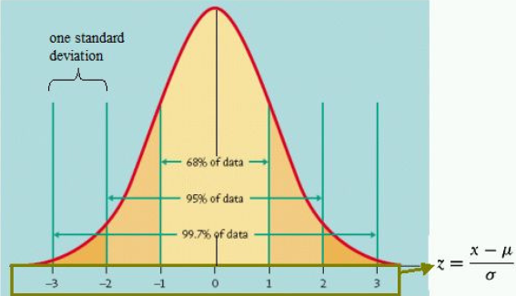
Let's illustrate the concept of mean and standard deviation with a simple example. My New York subway commute every day is 30 minutes on average, with a standard deviation of 5 minutes. Assuming a normal distribution for the time it takes me to get to work, this would imply that:
-
68% of the time, I can expect my daily commute to be between 25 minutes and 35 minutes (i.e., the mean of 30 minutes plus or minus 1 standard deviation, or 5 minutes).
-
16% of the time, my commute is less than 25 minutes (because the normal distribution is symmetrical around the mean, I expect this event to occur 16% of the time, or (100%-68%)/2).
-
16% of the time, my commute is greater than 35 minutes (again, because the normal distribution is symmetrical). Or, in other words, my 84% confidence level worst-case commute is 35 minutes (for example, only 16% of the time I would expect longer commute).
From this example, it makes sense that the more standard deviations we move from the mean, the lower the probability is of such an event occurring. For example, a delay of 10 minutes or more (2 standard deviations) only has a 2.5% chance of occurring, compared to a 16% probability of a delay of 5 minutes or more (1 standard deviation).
The table below relates standard deviations to lower tail probabilities (lower tail probabilities quantify the chance of an event of that magnitude or greater occurring):
| Standard Deviations | Lower Tail Probability | Commuting Example |
| 1 | 16% | Delay of 5 minutes or more |
| 1.28 | 10 | Delay of 6.4 minutes or more |
| 1.65 | 5 | Delay of 8.25 minutes or more |
| 2 | 2.5 | Delay of 10 minutes or more |
| 2.33 | 1 | Delay of 11.65 minutes or more |